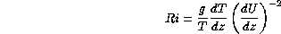
We have seen in section  that the effect of seeing can be quantified by the FWHM spread angle
  which can be evaluated as the integral along any given line of sight of
the local temperature structure coefficient
which can be evaluated as the integral along any given line of sight of
the local temperature structure coefficient 
(see section ).
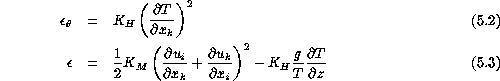
We will here describe how the temperature structure coefficient  is related to the quantities which characterize the turbulent velocity
and temperature fields.
is related to the quantities which characterize the turbulent velocity
and temperature fields.
The starting point is given by the relationship (),
derived by [Tatarskii] among others, which
relates 
to the dissipation rates of kinetic energy and temperature:
where  is a constant
equal to about 3.
is a constant
equal to about 3.
Introducing the eddy coefficients  for momentum and
  for temperature,
the respective dissipation rates can be expressed in tensor notation as:
for temperature,
the respective dissipation rates can be expressed in tensor notation as:
The last term at the right side accounts for buoyancy effects.
If the mean characteristics generally depend only on one geometrical
coordinate, as it is the case in a stationary atmospheric boundary layer
with the height z above the ground, the above expressions become:
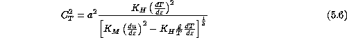
Inserting in ()
one gets:
[Wyngaard] has analyzed in detailed,
on the basis of experimental data, the parameterization of  in terms of the temperature and velocity fields in the atmospheric surface
layer using the so-called similarity theory.
in terms of the temperature and velocity fields in the atmospheric surface
layer using the so-called similarity theory.
Similarity theory is a method by which statistical mean and turbulent values in a flow/temperature field, when properly adimensionalized, are assumed to be universal constant or functions of a stability parameter. The adimensionalizing quantities, called scaling variables, and the stability parameter can be chosen in different ways by obeying to some simple rules (see for instance [Hull], pp. 347-361).
Here the scaling variables taken are the height z and the temperature
gradient  , while the Richardson
number was used for the stability parameter:
, while the Richardson
number was used for the stability parameter:
Noting that similarity theory predicts that  and
and  , hence
  , when adimensionalized are universal function of Ri, [Wyngaard]
derived the expression
, when adimensionalized are universal function of Ri, [Wyngaard]
derived the expression
The function f(Ri), obtained from experimental measurements is
plotted in fig.
and is a good illustration of the fundamental asymmetry of thermal turbulence,
hence seeing, with respect to the sign of the temperature gradient. As
a numerical exercise we have computed  by means of expression ()
as a function of
by means of expression ()
as a function of  for three
different speed rms
for three
different speed rms  values at 15 meters height above the ground (fig. ).
One will note that the effect of small variations of
values at 15 meters height above the ground (fig. ).
One will note that the effect of small variations of  on the local
  is very significant.
The achievement of low seeing implies very small temperature gradients,
particularly in unstable conditions. An exception is given by the case
of a stable gradient with low mechanical turbulence. This is possibly the
plainest demonstration that quiet inversion layers have very favorable
seeing characteristics.
is very significant.
The achievement of low seeing implies very small temperature gradients,
particularly in unstable conditions. An exception is given by the case
of a stable gradient with low mechanical turbulence. This is possibly the
plainest demonstration that quiet inversion layers have very favorable
seeing characteristics.
The variations of mechanical turbulence have opposite effects on 
depending if the thermal conditions are unstable or stable. For unstable
conditions and a same  ,
,  decreases with increasing turbulence. For stable conditions
increases dramatically with increasing turbulence. This means for instance that the artificial inversion obtained by chilling the dome floor in some observatories (CFHT, ESO 2.2-m) does achieve a low seeing only as long as no wind turbulence enters the dome.

Figure: The function f(Ri) in equation (5.7) - from [Wyngaard]

Figure: Computation of  versus
  in the atmospheric
surface layer, 15 m above the ground
in the atmospheric
surface layer, 15 m above the ground
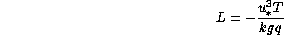
By choosing other scaling variables, namely the friction velocity  and the normalized surface heat flux q (in K m s
 ),
and as the stability parameter the ratio
),
and as the stability parameter the ratio  ,
where L is the Monin-Obukhov length
,
where L is the Monin-Obukhov length
[Wyngaard] obtains another expression
for  :
:
where  is an empirical
function evaluated from experimental data as:
is an empirical
function evaluated from experimental data as:
In presence of a strong turbulent flow, L is large and therefore  close to the surface is constant
  and equation ()
becomes:
and equation ()
becomes:
We note that this expression may be derived also directly from the general
expression ().
When friction effects predominate over buoyancy the second term of equation
()
may be neglected. Putting  we obtain:
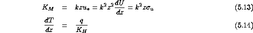
With this approximation and using a common parameterization for the K factors:
where k is the Von Karman constant ( 0.4),
0.4),  is the friction
velocity,
is the friction
velocity,  the velocity
rms and q the vertical heat flux, expression ()
can be elaborated as
the velocity
rms and q the vertical heat flux, expression ()
can be elaborated as
Near the surface the heat flux q is practically equal to the
surface flux  , which in
a turbulent surface layer is proportional to
, which in
a turbulent surface layer is proportional to  .
.
Therefore in a turbulent near-neutral surface layer  is proportional to
  hence
to
hence
to  which is the square
of turbulence intensity
which is the square
of turbulence intensity  .
One then finds that
.
One then finds that  is
directly related to both the squares of turbulence intensity and temperature
difference:
is
directly related to both the squares of turbulence intensity and temperature
difference:
 can also be put in relation
with the outer scale of turbulence
can also be put in relation
with the outer scale of turbulence  .
Following [Tatarskii], the outer scale of
turbulence is related to
.
Following [Tatarskii], the outer scale of
turbulence is related to  as
as
inserting this expression into ()
we obtain
The free convection case
When the flow is strongly unstable, that is when, approaching the free
convection condition, buoyancy predominates over friction effects such
that  , expression ()
becomes
, expression ()
becomes

inserting in equation ()and
using the definition of L, one obtains an expression in which  disappears:
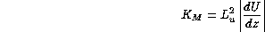
This relationship between surface flux, height and  is graphically illustrated in fig.
below.
is graphically illustrated in fig.
below.
Another expression for the free convection case can be obtained quite
simply from equation (),
noting that the function  becomes about 3.6 for
  (see fig. ):
which has the same form as equation ()
and where the distance z may be interpreted as a length scale parameter
which characterizes flow mixing in the free convection circulation process.
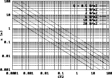
Figure: Relationship between  (K
(K m
m ),
height and surface heat flux in free convection over a horizontal surface
),
height and surface heat flux in free convection over a horizontal surface